Here’s a presentation by Prof. Emeritus Dr. Edward (Ward) Hindman of the Earth and Atmospheric Science Dept., The City College of New York, NY USA
www.sci.ccny.cuny.edu/~hindman
Presented at the SSA Convention, Reno NV, 2 February 2012
The Soaring Café thanks Prof. Hindman for providing the slides and script of his SSA 2012 presentation.
A slide-by-slide script of Prof. Hindman’s talk follows the presentation itself. Unfortunately, we do not have the video referred to in slide #2.
About the Presenter: CFI-G, glider owner, Gold badge, two Diamonds, developed meteorological instruments and conducted research, some for Paul MacCready between 1961 and 1964, in fogs, thunderstorms and hurricanes. Ward studied clouds at Storm Peak Laboratory (which he founded in 1981) in the air and at sea. During his 1995 sabbatical, he led a unique, transHimalayan, international expedition to Mt. Everest to study the feasibility of ascending Everest with a sailplane. At Colorado State University during his 2005 sabbatical, he investigated soaring flight using state-of-the-art atmospheric numerical models. He is continuing those studies and edits and publishes Technical Soaring.

Ward Hindman presents on "Modern Sailplanes Plus Extraordinary Weather Produce Extreme Flights"
VG01:
Good morning! I am Ward Hindman (hindman@sci.ccny.cuny.edu) of The City College of New York. I’m delighted to present ‘Extraordinary weather plus modern sailplanes produce extreme flights’. Here I focus on the weather and the weather predictions. The material used to make the predictions is mostly from the Internet and I display the web addresses. So, you won’t have to write down the addresses, this talk will appear on my web-site in the ‘Soaring meteorology’ folder. Warning, as I exhorted my students early in the development of the Internet, do not forget the tilde symbol (~) before ‘hindman’.
Here’s a nice photo of me and ‘Big Bird’ as my young children called my HP-14T.
VG02:
To get us in a good mood, this unique 3.5 minute video highlights the beauty and grace of soaring flight. The video was shot by Daniel Ramseier from an alpine peak near Dent de Broc during the 2004 Swiss National Championships. The alluring background voice is Enya’s. Enjoy!
VG03:
I am frequently asked ‘what keep these craft in the air?’ That is the main subject of this talk: rising air makes a glider a sailplane; and, the major sources of rising air for soaring flight are thermals, ridge winds and mountain waves. Then, I give examples of the extraordinary weather that produced extreme soaring flights: a thermal flight from Hobbs NM in June 2011 during the 18m Nationals, a ridge flight from Julian PA in April 2010 as reported in Technical Soaring [34(4), journals.sfu.ca/ts/] and a world-record wave flight in Argentina in November 2003 also reported in Technical Soaring [35(3 & 4)].
Here are two steps to answer the question ‘what keep these craft in the air?’
VG04:
First, we see the lift, weight and drag forces on a glider in steady-state flight. The lift and weight are at a slight angle producing a nose-low attitude and ‘thrust’. With an airplane, the lift and weight forces are directly opposed and the thrust is provided by an engine.
VG05:
Second, the glider’s thrust force is composed of the glider forward speed and the glider sinking speed. If the rising air speed is greater than the sinking speed, the glider is a sailplane; soaring flight occurs. Conversely, if the sinking air speed is greater than the glider’s sinking speed; gliding flight occurs.
VG06:
Here, the major sources of rising air that enable soaring flight are illustrated: thermals, ridge or slope winds and mountain lee- waves. The thermal wave, wave triggered by convection, is an infrequent phenomenon and, thus, has not led to extreme soaring flights.
Now, I will explain the extraordinary weather and the resulting extreme soaring flights.
VG07:
First, an extreme thermal flight on 26 June 2011 at the Soaring Society of America’s 18m National Contest at a hotter-than-normal Hobbs NM. Here you see the location of Hobbs – the red-dashed circle in SE New Mexico – and a view of the site.
VG08:
I will describe the morning weather forecast I gave to John Godfrey, the contest director, that was used, in part, to set the afternoon’s task: the winds at the surface and aloft, clouds and precipitation, convective boundary layer characteristics – depth and expected lift – and the possibility of thunderstorms. Then, I will illustrate the called task and the incredible results.
VG09:
The winds, clouds and precipitation came from the Terminal Aerodrome Forecast for KHOB (Hobbs/Lea County) and the high temperature came from the NWS local forecast. The expected surface weather: clear, windy and hot.
VG10:
The Satellite_Surface chart for 1030Z (0430MDT) on 26 June shows selected surface weather reports, radar echos (green), high-level clouds (white) and surface fronts (colored lines). At 0430MDT, a low was in the OK Panhandle with higher pressure in the contest region producing the weak southerly surface winds. Skies were clear in the SW USA. The dry-line, that separates the moisture-starved desert air from the moisture- filled Gulf air, is the diagonal dashed line through southeastern NM; the line moved from TX into NM overnight. The green radar echos over southeast NM and western TX are returns from the intense surface temperature inversion, not precipitation.
VG11:
The Upper Air Data at the 700mb level (about 10,000 ft MSL) for 00Z on 26 June (18MDT on 25 June) shows winds and temperatures: isotherms (yellow dashed lines) and 700mb height contours (white lines). It can be seen the ridge of high pressure was well established over the SW USA producing dry, subsiding air over the contest region. My morning forecast was made before the 12Z (06MDT) data were available.
VG12:
Here are the results from a numerical weather prediction model (based on the previous nights 00Z data) valid at 00Z (18MDT) on 26 June; the evening of the contest day. Shown are the expected surface isobars (blue lines), 1000-500mb thickness (yellow dashed lines) and precipitation (between 12 and 18MDT). At 18MDT, the surface low is expected to persist maintaining the warm, dry southerly winds at the surface. The upper- level ridge is expected to persist producing the southwesterly winds aloft over the contest region. Some precipitation is expected in northern Mexico and southwest TX but the blow-off from these storms should not affect the contest region. No precipitation is expected between 12 and 18MDT in the region.
VG13:
The so-called Meteorogram for Hobbs, valid between 12Z (06MDT) and 06Z (24MDT), from-top-to-bottom, shows expected winds at 700mb and at the surface, depth of the convective boundary layer (planetary boundary layer (PBL, m MSL)), cloud cover, precipitation and surface temperatures and pressure. The average PBL depth was expected to be 2500 ft AGL (~762 m, ‘trigger’ depth) at around 1000MDT (16Z) when the temperature was expected to reached 91F (33C). A PBL peak of 15,000 ft AGL (4600 m) in the average depth was expected between 15 and 18MDT (21-00Z). Because of expected cumulus formation, the average lift should be 10kts (2kts/1km PBL depth in clear skies, larger with Cu above). Winds at the surface and aloft were expected to be light from the southwest during the flying period. The maximum temperature of 108F (42C) was expected to be reached at about 14MDT (20Z) and persist to 18MST. No precipitation was expected.
VG14:
The forecast soundings at Hobbs for 12Z (06MDT) and 21Z (15MDT) show the expected vertical distribution of temperature (red line), dew-point (green line) and wind speed and direction. From these data, the probability of cumulus formation was estimated. The surface moisture was expected to diminish during the day due to mixing with the drier air aloft. This mixing was expected to produce afternoon, high-based cumulus capped by the significant temperature inversion at 500 mb generating ‘round, firm and fully- packed’ cumulus. The morning ‘jet’ from the southwest in the boundary layer winds was expected to mix away in the vigorous afternoon convection. The expected weak afternoon boundary layer winds and strong vertical mixing may make the cumulus scattered, not aligned in ‘streets’.
VG15:
Shown here is the expected horizontal distribution of the top-of-usable lift at15MDT derived from the Global Forecast System model. Hobbs is at the marker and surface winds are displayed. Thermals were expected to be deeper in the northern portion of the contest region. Top-of-usable lift at 15MDT was expected to be 14- 15,000 ft MSL. Thermals were expected to be deeper in the northern portion of the contest region. The same pattern was derived from the NAM and RUC models, but the NAM predicted the top-of-usable lift at Hobbs at 17-18,000 ft MSL and the RUC predicted 15-16,000 ft MSL.
These results were consisted with those from the meteorogram and I became quite excited about the possibility of a big soaring day!
VG16:
Before getting too excited, I checked for the possibility of thunderstorms that could easily ruin a day. Show here is the horizontal distribution of the Lifted Index (shows severity of thunderstorms) at15MDT derived from the Global Forecast System model. No storms were expected in the contest region because of the large index values though storms may form to the SE in the region of the negative index values, in the region of the Gulf Air.
[The Lifted-index at Hobbs at 15MDT is expected to be 0 to 1 (measures thunderstorm severity: > -3, weak; -3 to -5, moderate; < -5, strong). The values for the same index from the NAM model were 1 to 2 and the RUC model 0 to -1].
VG17: The task setters were excited, too! Task: 4.5 hours minimum time on course with 360 miles of required turn-points (Min: 172 miles, Max: 511 miles).
VG18:
In the days results from the SSA website, CD John Godfrey wrote “7V (70+ year-old Ray Gimmey) smoked the field with 465 miles at 103 mph”. I inspected his *.igc file and found he was 4hr 32min on course; 23% circling flight, 77% straight flight. Shown is his flight track.
VG19:
Here is his altitude track. Look at the incredible climb off tow. The CD launched the fleet after significant convection was underway to make sure pilots ascended quickly from the hellish ramp temperatures to the cooler air aloft. Look at the saw-tooth nature of the trace: ear-popping climbs in thermals and near red-line speeds between climbs. And, look at him bumping up against Class-A airspace!
VG20:
Here are my predicted ‘round, firm and fully-packed’ cumulus plus the panel of a competitor showing pegged variometers (> 1000 fpm climb passing through FL170).
VG21:
Now, we get back to earth with an extreme ridge flight that originated from Julian PA on 28 April 2010. The unique topography of the Appalachian Ridge and Valley System is illustrated. Quite a change from Hobbs!
VG22:
The pilot, 22-year old Devin Bargainnier flying a Ventus 2b, planned the flight because a cold front associated with a powerful low pressure system was expected to produce favorable winds for a large portion of the Appalachian ridge system between Williamsport PA and Knoxville TN. Further, the forecasts for cloud cover and precipitation for stations along the route were acceptable.
He did not utilize the experimental thermal, ridge and wave forecast system we – the German Weather service, the system’s creator Dr. Olivier Liechti and me – made available to northeast USA glider pilots during the 2010 soaring season. He was not aware of its existence. Had he used the system, this is what he would have learned.
VG23:
The forecast system is called Java TopTask. The system is operational in Europe through the German Weather Service (www.flugwetter.de) and is described in Technical Soaring [34(4)].
Briefly, the forecast system is based on numerical weather predictions of winds, clouds, precipitation, convective boundary layer characteristics and ridge and wave lift. The TopTask algorithm ‘flies’ a glider through the predicted weather to determine the feasibility of a proposed task. After the flight, the predicted weather can be validated by ‘flying’ the actual flight trajectory through the prediction.
VG24:
First, we inspect the thermal lift forecast for Julian PA (Julian is at the small red dot). Displayed on the map (left) are the expected winds and fight distances (km) for a 15m ship flying in randomly-spaced convective lift. It can be seen, the expected distances were only 100 km due to the strong winds. Displayed on the time-section (right) is the evolution of the convective boundary layer – lift between 0.5 and 2.0 m/s to 1500 m MSL – and the expected occurrence of low, middle and high clouds (L, M and W) and convective clouds (grey blobs). The initially overcast low clouds (8/8) were expected to become scattered (1/8) and form cloud streets after 10 EST while the middle clouds were expected to remain overcast (8/8). No precipitation was expected because no precipitation symbols are displayed.
Next, we inspect the ridge lift forecast. The ‘alignments’ switch was turned on and the expected flight distances increased dramatically to over 1400 km (gold diagonal line) due to the expected extensive, strong and long-duration winds perpendicular to the ridges.
VG26:
For the proposed task, an approximation of the actual flight track was traced on the map. The expected flight (the highlighted row in the upper left box) was 1520 km in length, flown between 0745 and 1844 EST at an average speed of 138 kph (77 mph). The expected flight profile is shown in the time-section with the stair- step red horizontal line. The flight begins in ridge lift when convection is expected to be weak, utilizes some convective lift mid-day and finishes in ridge lift at the end of the day when the convection weakens.
VG27:
Now, we input the actual flight track which is displayed as the red-black line on the map and as the jagged red-black line on the time-section. The length of the flight track (right vertical axis) is displayed as a function of time (horizontal axis). The slope of the straight diagonal line reflects the average ground speed of 155 km/h (86 mph) while the slope of the wiggly diagonal line gives the instantaneous ground speed: fast in the ridge lift and slower in the convective lift. It can be seen the flight began at ridge-lift altitude, went temporarily into wave lift (circle), came back to mixed ridge and convective lift and finished in ridge lift.
VG28:
The validation of the forecast for thermal and ridge lift is shown here. The recorded flight is displayed both on the map and in the time-section. It can be seen in the time-section, the simulated flight profile followed well the recorded track except the brief climb in wave lift. The simulated ground speed is 8% slower than the ground speed of the real flight (155 vs 142 km/h). These results illustrate the forecast verified.
VG29:
What result would have occurred had the pilot remained in wave? To answer this question, both the ‘alignments’ and ‘wave’ switches were activated. The simulated flight profile in wave is the red, stair-stepped horizontal line in the time-section. The overlapping diagonal lines illustrate the ground speed of the simulated flight is almost identical to the ground speed of the real flight. This result suggests that the flight might have been as successful in wave.
I learned from Devin long-distance flight in wave was not possible: “I chose to use the wave”, he reported, “because of the ease of entry. I exited wave when it became unorganized as a result of poor upwind ridges and almost complete cloud cover below. I descended through a small gap in the cloud cover and continued the flight in ridge lift and thermals.”
VG30:
Pilots participating in our experiment provided positive and encouraging evaluations. Consequently, Dr. Liechti and I attempted to make the JavaTopTask forecast system available the 2011 soaring season. The system needed to be connected to an operational USA numerical weather prediction model to replace the unavailable German model. No connection was made because the necessary expert could not be found. Hence, the system was and remains unavailable.
Baud Litt reported – in the recent issue of the National Soaring Museum Journal [33(2)] – pioneering long- distance flights in convective, ridge and wave lift during the winter of 2010-11 similar to the flight simulated here. Baud’s flights originated from Fairfield PA in the Appalachian Ridge and Valley System. Had the forecast system been available to study Baud’s flights, the TopTask algorithm would have benefitted especially the wave portion.
VG31:
Finally, I describe Klaus Ohlmann’s world-record, straight-line, Kuettner prize-winning wave flight of 2138 km (1188 mi) from El Calafate in extreme southern Argentina to San Juan in northern Argentina on 23 November 2003 in a Nimbus 4DM with co-pilot Herve Lefranc. The flight is described in Technical Soaring [35(3 & 4)].
VG32:
The weather forecast required to set the task was provided by the Mountain Wave Project team (www.mountain-wave-project.com). The forecast consisted of the following elements: winds aloft, clouds and precipitation and wave lift.
VG33:
As for the winds aloft, the Polar Front Jet Stream and the Subtropical Jet Stream were juxtaposed ‘hosing down’ the maximum length along the Andes. Notice the Polar Front jet was aligned S-to-N in Patagonia but still crossed the Andes because there they curve to the SE.
VG34:
As for clouds and precipitation, the altocumulus standing lenticular clouds above and rotor clouds below marked the wave. The clouds were too thin to produce precipitation.
VG35:
To locate the wave lift, the pilots ‘read’ the clouds. As illustrated here, the lift is along the windward face of the high Altocumulus standing lenticular clouds and the rotor clouds below. They essentially ‘surfed’ the wave like the familiar surfer riding the face of a gigantic breaker.
VG36:
Here is the altitude trace of the flight, the flight statistics – 2138 km (1188 mi), 14.5h, 147kph (82mph), 10% circling & 90% straight – along with significant photos and statements by Ohlmann.
VG37:
As a result of this successful Kuttener Prize 2000 km straight line flight, the Kuettner Prize 2500 km straight free-distance flight was recently announced in Technical Soaring [35(3)]:‘Since it is considered possible to achieve the 2500 km free straight distance in soaring flight with high performance sailplanes by using only meteorological power sources such as waves, cloud streets, slope winds etc. combined with meteorological navigation and flight techniques, OSTIV continues to comply with the wish of the late Dr. Joachim Kuettner to set up a prize and trophy for the first flight over the 2500 km free straight distance.’
VG38:
So, now you know rising air makes a glider a sailplane and you know the significant sources of rising air: thermals, ridge winds and waves. I showed you how extraordinary weather plus modern sailplanes piloted by world-class athletes-of-the-sky produced an extreme thermal flight from Hobbs NM in June 2011, an extreme ridge flight from Julian PA in April 2010 and the Kuettner Prize flight in an extreme wave event in Argentina in November 2003.
Now, go plan and achieve your extreme soaring flight. Amen! 6