Should Darwin’s Theory need to be proved any further, we can’t think of a better method than conceiving an algorithm able to mimic the fundamental mechanisms of natural selection and set it at work to produced highly adapted solutions. This is exactly what in the mid-seventies. Prof. John Holland did, by laying the foundations of what today is one of, if not “THE”, most powerful optimization tool available to scientists and engineers: the Evolutionary Algorithms. Prof Holland didn’t pursue the idea of giving a further proof of the Darwinian intellectual masterpiece, but he rather argued that the evolution process taking place in Biology is nothing but a mighty optimization process, able of moulding the DNA of living creatures so that they eventually adapt to their own environments. He was quite right! Not only because looking at how dolphins and sharks swim or (to stay closer to topics dealt with in this Cafè) Albatross soar you would also have to conclude that they’re perfectly engineered machines, but mostly because EAs (also known as Genetic Algorithms, GAs) are nowadays applied in any science field where optimal solutions to complex problems are sought. Complex problems are those dominated by a large enough set of parameters such to make very hard finding combinations of those which would result in optimal solutions to the problem itself. If you’re now wondering what this whole story has to do with gliders and their airfoils, well, you’ve probably never tried to design one. In fact airfoil design is another engineering task which falls in the above mentioned set of complex problems, especially when it comes to design wing sections for a competition glider. GAs are nowadays routinely and extensively used in the aeronautical industry. They are applied in aerodynamics as much as in structural design, many times in both fields at the same time, pursuing what is called MDO, Multi-Disciplinary Optimization. However such a technology is not yet available to the small, and medium, aircraft manufacturers. The mission at Evolution Designs is to fill the gap. Feel free to visit our web site at www.evolutiondesigns.eu

In this article it will be shown how EAs work in EDGAR, a software engineered to design optimal wing sections. Before setting off with a challenging enough test of the method let’s have a little more insight in the analogy with the natural evolution that form the backbone of a EA. In this analogy the parameters defining our solutions are regarded as the DNA of the solutions themselves. A solution is an individual and as in the nature, in a EA a whole population of solutions exists and struggles against the “pressure” of the surrounding environment. The “environment” is defined by the designer by setting the optimization goals (rarely only one). The best adapted solutions shall be those able to satisfy to those requirements and accordingly they will enjoy a higher probability to transmit their DNAs to the next generations. If you ever wondered why regnant throughout the history of mankind happened to have so many off-springs (sons and daughters, mostly illegitimate) that’s the reason! We said before that an EA mimics the fundamental mechanisms of the natural evolution. These are essentially: mutation, perturbation, selection and reproduction. The first twos act by introducing mutations and perturbations into the DNAs in a completely random fashion. Mutations and perturbations are occurring in nature as you read. They are the real “innovators” in the whole process. The selection does what a selection is supposed to do: it ranks and selects the most adapted solutions for mating. If you ever wondered why Marilyn Monroe ended up having love stories with Joe di Maggio and J.F. Kennedy but not with you, by reading this far you should have finally got it! Finally the reproduction creates the new generation where the parents’ DNAs end up mixing together somehow. That “somehow” has been subject of an extensive research in the EAs community but this’s not interesting in this context. Another thing that EA share with the natural evolution process is the enormous amount of combinations tested over the generations. This is in facts what makes a GA so much more powerful than any experienced designer can be. On a current desktop computer tens of thousands of solutions, in this case airfoils, can be generated, evaluated, ranked and selected in a matter of a few hours. Last but not least, if the natural evolution set off around 4.5 billions years ago starting with a nothing more than a mono-cellular living creature, so does in a way a GA, as it doesn’t need to start with any set of good wing sections to make them outstanding. This translated for the airfoil designer means that he doesn’t have to have access to any airfoil database to design an outstanding wing section. So, if you’re now wondering what the designer is left to do if EDGAR is installed on his computer, well this time we share your bafflement. At this point we’re ready to test what GA’s are really able to do and in order to do this for real we’ve to pick up a true “champion” to compete against. We selected the airfoil DU97-127/15M (Delft University, 12.7% relative thickness, 15% flap chord), the airfoil of the ASG-29 wing. The measured data of this airfoil are published on a technical article presented at the NVvl a few years ago.

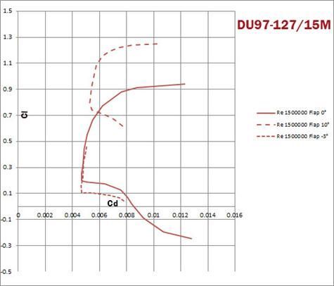
The wonderful job done with this airfoil appears at the first glimpse. The laminar intervals stretch to their maximum. As a matter of fact the ASG-29 shows at the top of all the competition rankings in 15 and 18 meters classes.

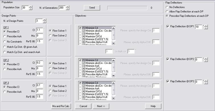
In order to design an airfoil for a given glider, one should figure out the lift distributions at the most significant speeds ( i.e. wing loadings) and flap settings for basically the climb and the inter-thermal flight phases. We want to stress here that designing an airfoil only for climb will result in a poor max (L/D) ratio at the inter thermal flight and vice versa, designing only for L/D will end up in a poor climb index, i.e. climb performance. This “competition” of the requirements is nothing but the norm in airfoil design as in any other engineering problem solving task. Another great deal in using GAs coded in a multi-objective fashion, as EDGAR is, is that the optimal solutions will be presented on a map which highlights immediately the trade-offs of selecting one specific wing section. Back to the design objectives, as we have a term of comparison, we shall limit ourselves to generate an airfoil which has as much an extended laminar interval as the reconstructed DU97-127/15M but possibly featuring less drag. We pick therefore the corner points of the laminar region of the polar with zero degrees flap, namely Cl = 0.2 and Cl = 0.7 at Re = 1.5 m. and the upper corner point of the polar with 10° flap, Cl = 1.1 again at Re= 1.5 m. and we will simply ask EDGAR to minimize the drag at those conditions. Now that we have specified a few objectives we’re ready to run EDGAR. Let’s do it then. The main GUI will prompt. By clicking on the “New Run” button a brief procedure for setting up the evolution will start. In the first window the user is asked to specify the population size, the number of generations to evolve the flight conditions and the objectives, plus in this case the flap deflection to be used at each condition.

By clicking on the “next” button twice one reaches to the parameters dialog. Through this form one can specify the range of allowed variation for each parameter defining the shape of an airfoil. Should one still doubt that the wing sections of a competition glider are something really special, a specific parameterization, that no other airfoil type shares, was implemented in EDGAR in order to generate “state of the art” wing sections for this application. In order to call it up let’s press the button “Sailplanes” and let’s leave the default radio button “Race gliders” checked. Only a few more clicks are still needed. First of all, as the selected champion has a 12.7 relative thickness, we have to fix the min. and max. values of the respective parameter to the same value. By doing so the range of variation of the relative thickness shall be zero and only 12.7% thick airfoils will show up during the evolution. The other parameter ranges were already tuned by pressing the “Sailplanes” button so we don’t need to touch them.

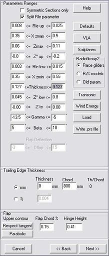
As you can see the DNA of an airfoil is pretty simple. It consists of around ten parameters such as: nose radius, station of the max thickness, relative thickness, upper and lower contour curvatures and finally the two trailing edge exit constructive angles. As simple as it can be any minimal change in each of these parameters is able to produce an airfoil whose aerodynamic characteristics are completely different from the starting one. Thanks Prof. Holland for giving us the EAs! We’re still left with specifying the trailing edge thickness, zero for this exercise, the flap length in percent of the airfoil chord, 15% in the case of the DU97-127 and the height of the hinge point in percent of the local airfoil thickness (41%???). A few words about the buttons “Respect Tangent” (default) and “parabolic” must be spent. By pressing them the user dictates the shape of the flap upper contour. The default condition “Respect tangent” shall produce flaps whose upper contour is aligned with the upper contour airfoil tangent at the hinge station when the flap is deflected by 10°. This should produce an as smooth as possible contour and pressure recovery with a flap deflection which is typical for climbing in a thermal. The resulting flap contour will be slightly S-shaped. Should this represent a constructive inconvenience the button “Parabolic” shall impose the upper contour to respect only the trailing edge constructive angles, resulting in a monotonic second derivative.

We’re ready now to proceed. Let’s press once the “next ” button at the bottom of the form. The process is going to be completed and the run is going to start in a matter of seconds. Just let’s specify the boundary layer transition points for the upper and lower contours. “1” means free transition. On the lower contour we set 0.95. This is done because the reference airfoil has turbolators at that chord station. Even if we wanted to run a completely independent optimization session we had to recall that the modern airfoils for competition gliders manage to keep laminarity on the lower side up to about 95% of the chord. Quite remarkable! However at that limiting station we want to trigger the transition somehow in order to avoid the rising of a laminar bubble, which would otherwise eat some performance. This is why modern gliders have turbolators at around 95% on the lower wing surface, whereas less modern gliders show turbolators somewhat more upstream, typically ahead of the flap hinge line, therefore at around 80 – 85% of the chord. How far the turbolators show up on a wing is an index of how sound its airfoil design is. By pressing twice more the “Next” button we are done with the setup and ready to launch the evolution. Please note that the time to set up the run was not more than a couple of minutes. Now we have to wait a little more for the GA in EDGAR to do its job.

 

…A couple of hours later…

 

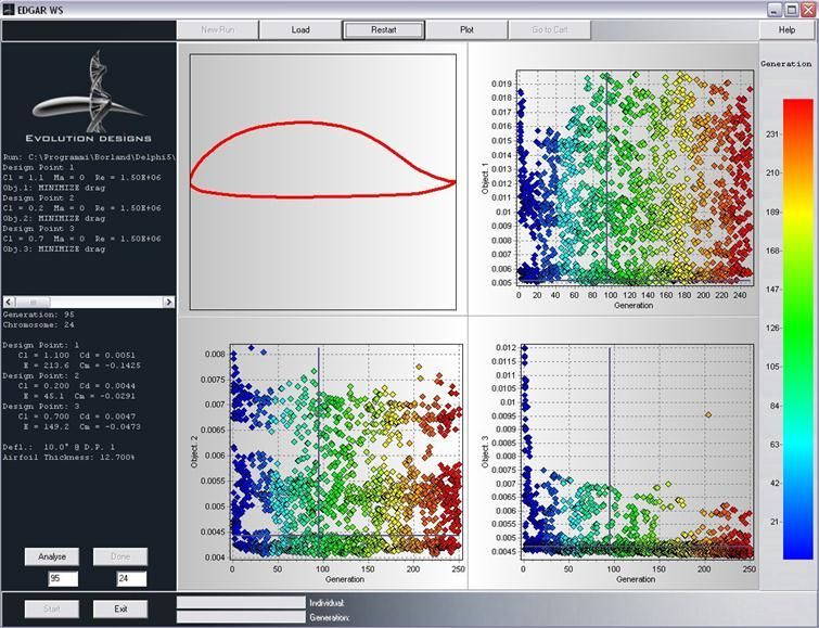
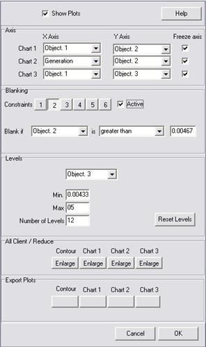
Ok, the GUI looks now pretty crowded and messy. First of all each dot represents an airfoil which was among the best one at least at its generation. By clicking on any of them a pseudo-contour of that particular wing section is drawn on the left upper display and the GUI is ready for analyzing. As there may very well be thousands of dots you may want to do some order. In order to do so, press the “Plot” button. In the form that pops up let’s select to show in the first solution panel (second display, up) the objective 2 against the objextive1. As the objective 1 and 2 were “minimize Cd” at the first and second design point what oyu’re watching now are the Cds at design point 1 (x axis) and at design point 2 (y axis). It still looks pretty messy but by zooming the bottom left corner (drag a square while pressing the left mouse button) some pattern starts showing up. Let’s do the same with last solution panel and display objective 3 against 1.

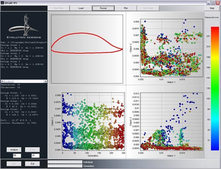
It should now be possible to spot the good solutions hiding in the clouds. The goods solution in this exercise are those featuring less drag than the DU97-127/15M at the respective design points. Please recall now what was stated before about the “competition” of the objectives. If you click on the best solution appearing in the first panel you will see that the corresponding dot in the third panel is probably much worse in the third objective.

In order to be able to dig the real good solutions out of a ordered but still crowded cloud let’s use the “blank” buttons and blank out any solution whose Cds are higher than those of our champion.

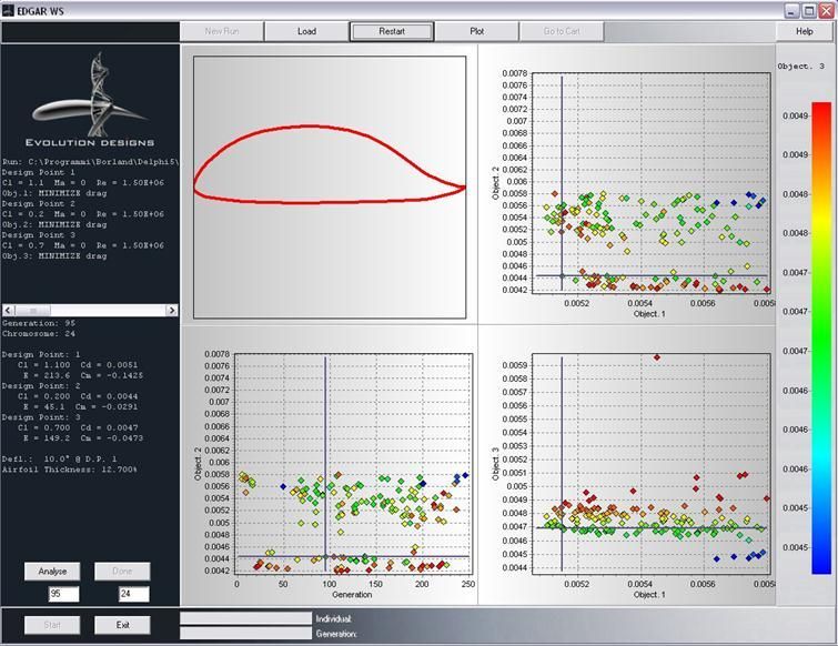
Any dot left in the net, if there is any, points to a very good indeed candidate. The one labeled as “Gen095_024of30″ (generation 95, individual 24 out of a 30 individuals population” looks very promising. Let’s select it and get ready for some analysis. On the left black panels the values of the aerodynamic coefficients are printed for each of the design points. The drag at climb (DP1) is 0.0051, i.e. -12.2% less than that of the DU97-127/15M, which translate into a power factor (Cl^1.5/Cd ) 13.8 % higher. At design point 2 the Cd is also lower by 6.4%. The new airfoils shows a pronounced laminar bucket which extends from the lower usable end of the polar up to Cl 0.8. Finally at lift coefficient for DP3, 0.7, EDGAR was able to reduce the drag by 17.5% or in a turn a L/D ratio increased by 21.3%. At this point it must be recalled that we’re comparing experimental data, those of the DU97-127/15M with analytic results. However, the most common available prediction methods can calculate the flow characteristics of an airfoil fairly accurately. Whether the experimental data where measured in a somewhat high turbulence wind tunnel and/or the predictions are somewhat optimistic, the numbers above let believe that more than a few percentage points of improvement can still be achieved over an already outstanding airfoil.

Having said this, Gen095_024of30 is definitely a guy we want to analyze more thoroughly. By pressing the “Analyse” button the “Analysis” dialog pops up. One can perform point analysis or sweeps in alpha, Mach (not interesting for gliders) and Reynolds. Let’s do a point analysis first at the design points.

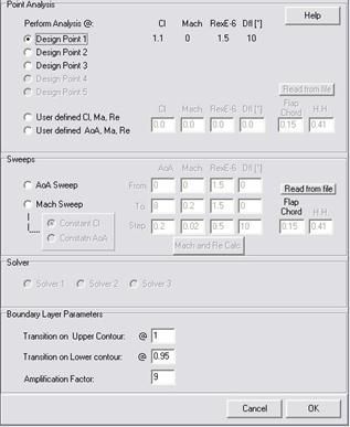
The first DP is already selected by default in the upper half of the panel and the respective flight condition is highlighted. By checking the other radio buttons the airfoil will be analyzed accordingly. Press the button “Analyse” at the panel’s bottom and a few seconds later the pressure distribution will appear and superimposed to the pseudo-contour.

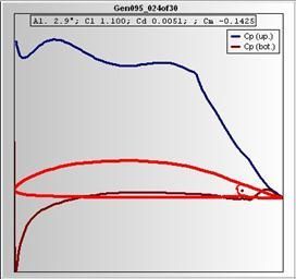
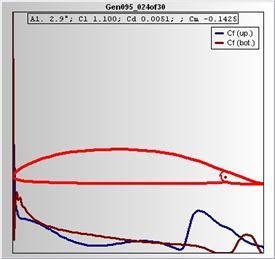
The pressure distribution at DP1 (flap deflected by 10°) around 85% of the chord looks smooth and almost undisturbed at the jump from the fixed to the movable part of the airfoil. Of course EDGAR assumes that a tape would be there sealing the gap. At the bottom of the main GUI a radio button allows to switch to the friction coefficient visualization. It looks like the airfoil is able to maintain laminarity all the way up to …% on the upper contour and to the 95% on the bottom.

Finally the designer may want to produce sweep in alpha. The central part of the analysis panel is pretty intuitive. After a few the polar will be displayed and the values of Cl, Cd and Cm will be automatically dumped in a .swp file in text format. The calculated polar where collected and plotted against the experimental data of the DU97-127/15M and are presented hereinafter

 

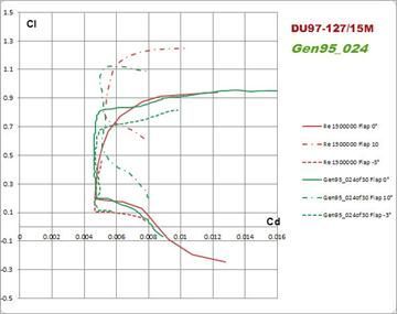
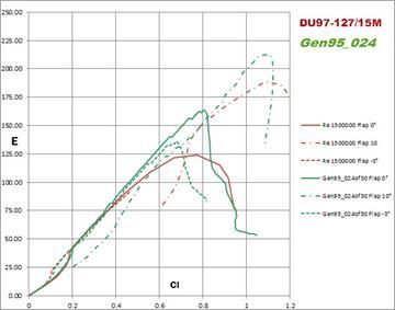
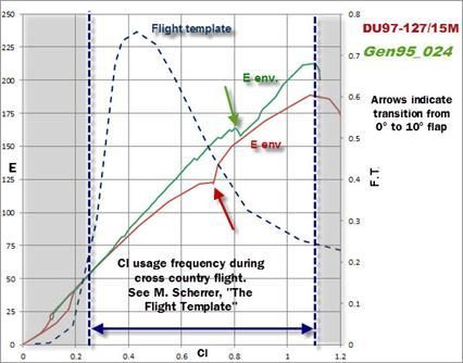
The envelope of E as a function of Cl in the previous picture shows a smoother transition from flap 0° to 10° while reducing speed. It is also interesting to relate the Efficiency envelopes of the two airfoils to the blue dashed line: the Flight Template. The flight template was derived by Matthieu Scherrer and represents a statistical distribution of the pilots usage of the lift coefficient during cross country flights. The probability to fly between Cl1 = 0.4 and CL2= 0.7 is given by the integral of the FT curve calculated between 0.4 and 0.7. According to the shape of the curve this probability is higher than that of flying between Cl 0.8 and 1.1. Please note that the FT is referred to the glider lift coefficient, thus to the CL. As the modern gliders have a wing planform that closely approximate the elliptic one, the section lift coefficients Cls across the span can be assumed to take the same value of the glider total lift coefficient CL.

Conclusions. With this simple exercise it was shown that designing in house an excellent airfoil is nowadays possible for the glider manufacturers with ease thanks to the extremely powerful method which was implemented in EDGAR. Most importantly it can be done in a matter of hours on a modern Windows PC, mostly spent by the GA. The designer is left with the task of carefully assign the optimization objectives and, at the end of the run, to go hunting for the best airfoil. By recalling the result of the Flight template theory, it as assumed.

Without forgetting that in this exercise analytic results where compared with experimental data, the comparisons show that some improvements of state of the art airfoils such as the DU97-127/15M may be possibly still achieved. This is not a negligible opportunity in the business of manufacturing competition gliders especially in the light of the fast growing interest that this wonderful sport is attracting. At Evolution Designs we will be proud to bring your gliders to be at the top of performance.

 

ED’s Team

info@evolutiondesigns.eu

www.evolutiondesigns.eu